Loading
The Silent Failures Killing Your ML Models (And How to Fix Them)
Why training-serving skew, data leakage, and irreproducibility share the same root cause, and what a feature store does about it.

You’ve been there. The model scores beautifully in evaluation, 94% accuracy, clean metrics, everything looks great. You push it to production. A week later, something feels off. Predictions are wrong, but there’s no error, no stack trace, nothing to debug. The model just quietly… fails.
This isn’t a model problem. It’s a pipeline problem.
Three symptoms, training-serving skew, data leakage, and irreproducibility, tend to be treated as separate issues. They’re not. They’re all expressions of the same underlying design failure: the absence of a single, well-governed source of truth for your features.
This article walks through how a feature store solves all three, what a production-ready reproducible pipeline looks like in practice, and the non-negotiable rules that keep ML experiments trustworthy.
The Three Faces of the Same Bug
Training-Serving Skew
Your training pipeline is built by one engineer. You’re serving pipeline by another, months later, possibly in a different codebase. They both think they’re computing the same features, but small differences accumulate. A different normalization range here, a slightly different aggregation window there. By the time the model reaches inference, it’s receiving inputs it was never actually trained on.
The frustrating part: this doesn’t throw errors. The model just silently receives wrong inputs and produces wrong outputs.
Data Leakage
Leakage happens when your model learns from information it wouldn’t have at prediction time. There are two classic forms:
Target leakage: a feature that directly encodes the label sneaks into training. Imagine predicting gym subscription cancellations and accidentally including a column called reason_for_cancellation. Your accuracy looks incredible. Your model is useless.
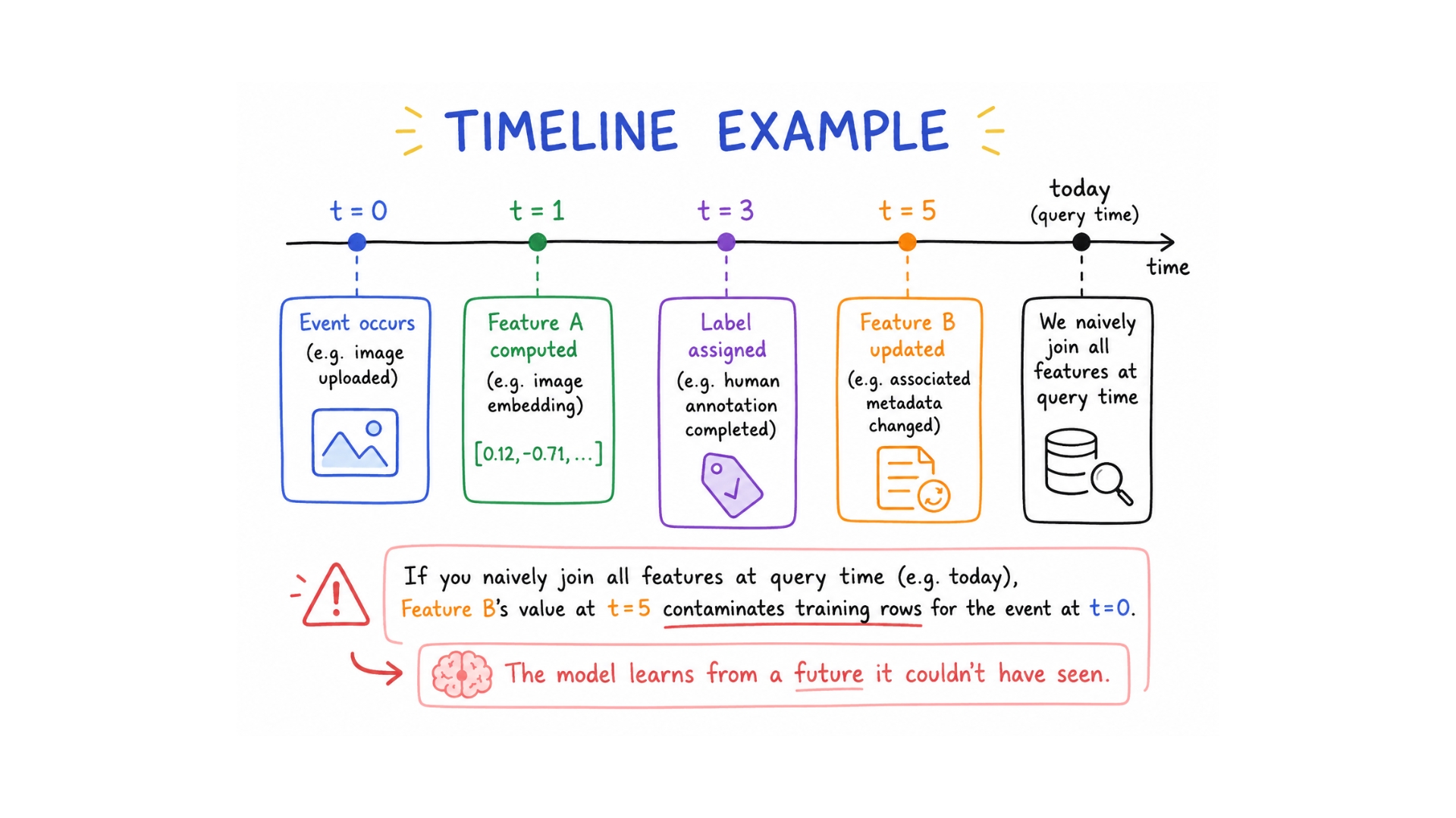
Temporal leakage: future data is used to predict the past. You’re training a model for a June event using a feature value updated in December. In production, that December value doesn’t exist yet.
For image data specifically, the risks multiply: augmenting before splitting (so augmented variants of the same image appear in both train and test), near-duplicate images bridging splits, or EXIF metadata (device IDs, GPS coordinates, timestamps) correlating with labels in ways you never intended.
Irreproducibility
You ran an experiment last month that got great results. Today, you can’t reproduce it. Your teammate runs the same code on “the same” data and gets different numbers. Retraining gives different outcomes.
The cause is almost always the same: the dataset, preprocessing state, and environment weren’t versioned together. Code versioning alone isn’t enough.
What a Feature Store Actually Is
Think of a feature store as a shared library for your features, a system that manages creation, storage, and serving of features consumed by both training and inference from a single source of truth.
This is the key insight: if training and serving both read from the same store using the same computation logic, skew becomes structurally impossible.
A feature store does four things:
- Stores precomputed features with timestamps and metadata, not just the values, but when they were computed and from what source.
- Serves features to both offline training pipelines and online inference, with the same definition and two materialization targets.
- Tracks feature lineage, who created this feature, when, and from what raw source.
- Enables point-in-time queries, preventing temporal leakage at the infrastructure level.
The Two Layers
A feature store has two storage layers, and understanding the distinction is critical:
| Offline Store | Online Store | |
| Used for | Training | Inference |
| Latency | Minutes | Milliseconds |
| Query pattern | Historical range scan | Single entity lookup |
| Storage | Data warehouse / object store | Low-latency DB (Redis, DynamoDB) |
The same feature computation logic populates both. Features are materialized from offline to online, so at inference time, they can be retrieved in milliseconds. Zero divergence. Zero skew.
Point-in-Time Correctness
This concept is worth its own section because it’s the mechanism that kills temporal leakage at the root.
The rule is simple: every training sample must use only feature values available at the moment the sample was observed, never values updated afterward.
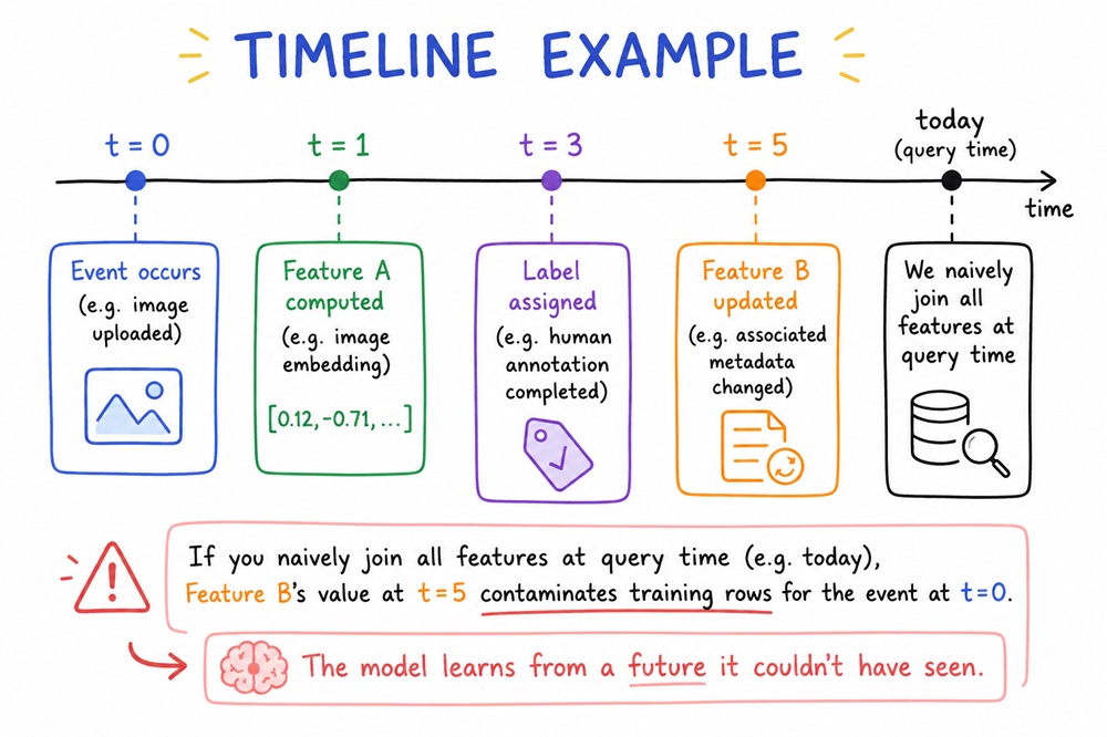
Timeline Example
Concretely: if a feature was set at time T1, and later updated at T2, and your training sample was observed between those two times, the point-in-time join returns T1, not T2. The model trains on what was actually knowable at that moment.
Feature stores make this automatic. Every feature lookup is anchored to the sample’s observation timestamp. You’re not relying on engineers remembering to be careful; the infrastructure enforces correctness.
This matters especially for image pipelines. Consider a computer vision model in which images are labeled at ingestion and then re-annotated by human reviewers hours later. The label used for training must be the one from the original observation, not the reviewed version, because at inference time, that review hasn’t happened yet.
One Pipeline, Five Stages
Here’s what a reproducible ML pipeline looks like end-to-end, built around the principles above. The stack: MinIO for object storage, Feast as the feature store, MLflow for experiment tracking, Redis as the online store, and DVC for data versioning.
None
feature-store-demo
├── infra/
│   └── feast/
│       ├── feature_store.py
│       └── feature_store.yaml
├── pipeline/
│   ├── 01_ingest.py
│   ├── 02_clean.py
│   ├── 03_extract_features.py
│   ├── 04_create_dataset.py
│   ├── 05_train.py
│   ├── 06_serve.py
│   ├── 07_reproduce.py
│   ├── extract_utils.py
│   └── utils.py
Stage 1: Ingest & Store
Raw images arrive from a source, a camera, a scraping job, or a dataset download and are uploaded to an immutable bucket in MinIO. Stable image IDs are generated at this point. A manifest (raw_manifest.json) is created capturing image_id, minio_uri, label_at_ingestion, and ingestion_timestamp.
The label captured here is the label at ingestion time, not a later re-annotation. This is intentional.
The golden rule starts here: raw data is never modified. Every transformation produces a new, versioned artifact. If a cleaning bug is discovered three weeks later, you fix the cleaning stage and re-run from raw. Nothing is lost.
Stage 2: Clean & Validate
The cleaning stage reads from the raw manifest, downloads images, applies resolution validation and deduplication, and writes clean images to a separate clean-images bucket. A new manifest tracks total_raw, total_clean, total_quarantined, and cleaning_version.
Keeping raw data untouched is what makes mistakes survivable. Fix the broken stage, re-run from the original, every downstream artifact regenerates cleanly. Overwrite the source, and there’s nothing to recover from.
Stage 3: Feature Extraction + Feast
Clean images are downloaded, embeddings are extracted using a pretrained embedding model, and the results, along with metadata, are written to feast_features.parquet. Feast registers the feature views and materializes features into Redis (the online store).
What goes into the feature store: URI + embedding + label + ingestion_timestamp + preprocessing_version. The preprocessing version matters: if your embedding model or normalization logic changes, you’ve effectively created a new feature. Old versions must be preserved.
Stage 4: Point-in-Time Dataset
This is where Feast earns its keep. The get_historical_features function performs a point-in-time join, filtering entities according to a configured cutoff timestamp. Train, validation, and test splits are created and saved as a versioned dataset:
None
dataset_v1.0_pit_.json
dataset_v1.0_pit__data.parquet
The JSON manifest captures dataset_id, content_hash, cutoff_timestamp, split_counts, and extraction_model. This is the artifact that makes experiments reproducible.
The pipeline also supports a –leaky flag that creates a separate dataset without point-in-time correctness, useful for demonstrating exactly how much leakage inflates your metrics.
Stage 5: Training + MLflow
A LogisticRegression model is trained on the embeddings. Everything is logged to MLflow: parameters, metrics, the model artifact, and crucially, dataset_id, dataset_content_hash, and dataset_cutoff. Every run is traceable back to the exact dataset version that produced it.
Stage 6: Serving
At inference time, online features are retrieved from Redis through Feast, the same feature definitions used during training, now served at millisecond latency. The model registered in MLflow is loaded, and a prediction is run.
This closes the loop: the same feature computation logic that populated the offline training store now powers real-time inference.
Stage 7: Reproduce a Run
Given an MLflow run ID, this stage reads the run metadata, recovers the dataset version used, and validates that the run has enough traceability to be reproduced. dataset_id, content_hash, code version, and parameters are all connected.
Dataset Versioning Is Not Optional
Model versioning, saving weights, architecture, hyperparameters is widely adopted. Dataset versioning is not. This asymmetry causes most reproducibility failures.
A comprehensive dataset version captures:
- List of sample IDs included, every data point is accounted for
- Cleaning + feature extraction code version, data is linked to the exact code that transformed it
- Model/library versions for embeddings, external dependencies used in data creation, are documented
- Train/val/test split assignments + seed, identical splits guaranteed across runs
- Content hash, a unique identifier verifying the dataset’s immutability
DVC handles this in the demo pipeline. Combined with MLflow’s experiment tracking, every model run is connected to a specific, reproducible snapshot of the data.
Images Amplify Every Challenge
Tabular data has its reproducibility challenges. Image data makes all of them harder:
Scale, millions of high-dimensional files require storage strategies that simply don’t apply to CSV data. Raw images live in object storage (MinIO/S3). Embeddings and metadata live in Parquet files. These can’t be collapsed into the same artifact.
Feature diversity, for tabular data, features are columns. For images, you have semantic embeddings, bounding boxes, masks, resolution metadata, EXIF data, each requiring different handling and versioning.
Preprocessing sensitivity, a different resize method, normalization range, or color space conversion can meaningfully shift your data distribution. These choices need to be versioned.
Embedding versioning, any change to the embedding model or the library version creates a new feature. The old embeddings must be preserved; you can’t recompute them without reprocessing every image.
The Five Rules
If you take nothing else from this, take these:
- Write features once. Use a feature store for both training and serving. Never duplicate transformation logic across pipelines.
- Never overwrite raw data. Every transformation creates a new versioned artifact. Immutability enables safe re-runs and late bug discovery.
- Always respect time. Use point-in-time joins. Every feature lookup should be anchored to the sample’s observation timestamp.
- Version everything together. Data + Code + Environment + Splits. Model versioning alone is not reproducibility.
- Close the loop. Every experiment must be traceable back to its exact dataset. If you can’t answer “what exact data produced this model?”, your pipeline isn’t production-ready.
The infrastructure described here, Feast, MinIO, MLflow, Redis, DVC, all wired together in Docker, is not exotic. It’s the minimum viable stack for taking ML reproducibility seriously. The concepts apply regardless of your specific tooling choices.
The real shift is architectural. It’s the decision to treat features as first-class artifacts with lineage, timestamps, and versioning, not as ephemeral transformations scattered across notebooks and ad-hoc scripts.
When training and serving pipelines share a single source of truth, and every dataset is a versioned, hash-verified artifact linked to the model run that used it, silent failures become diagnosable. Experiments become reproducible. Production becomes trustworthy.
That’s the whole point.
The complete pipeline code referenced in this article, including all seven stages, Docker Compose configuration, DVC setup, and the PIPELINE_GUIDE.md, is available in the feature-store-demo repository.